by Tim Blömeke

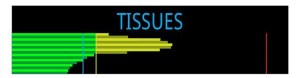
If you’re the owner of a Shearwater dive computer and clicked through the info screens, you may have seen this:

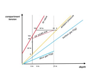
And if you’re a technical diver using the Bühlmann ZHL-16C algorithm, then I’m certain you’ve seen some kind of visualization of M-values and gradient factors (GF) according to Erik Baker:

In this blog post, I would like to take a minute and explain how the two are connected.

First, let’s take a look at the Shearwater compartment graph and how the manual explains it.

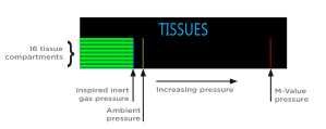
The graph displays all of the 16 compartments and their inert gas tensions relative to inspired inert gas pressure, ambient pressure, and M-value.

When the inert gas tension is below ambient pressure, the compartment bar is green. For compartment tensions above ambient pressure and below the M-value (positive GF between 0 and 1), the compartment bar is yellow. Above the M-value (GF > 1, not recommended), the bar turns red.

The cyan (blue) vertical line indicates the inspired partial pressure of inert gas P(ig). All of the (theoretical) compartments converge on this limit at different rates over time from either side, and you can see if a compartment is (theoretically) on or off-gassing.

Please note that since M-value parameters (zero pressure crossover a and gradient b) are different for each compartment, the graph does not scale perfectly.

In a Baker-esque diagram for a single compartment, the areas look like this (same-ish color coding):

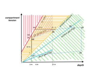
The section cross-hatched in both yellow and red (top center, above the GF line and below the M-value line) is not indicated separately in the “Tissues” graph. That is, the Shearwater graph does not account for personal gradient factor settings – even though the computer will of course calculate deco based on your configured limits and warn you if exceed them.

In fig. 5, you may have noticed a thin blue line with numbers from (1) to (6). This line shows the path of a single compartment (simplified) as the dive progresses.

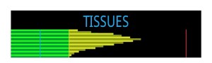
The Shearwater graph does a similar thing in real time during a dive, for all 16 compartments:

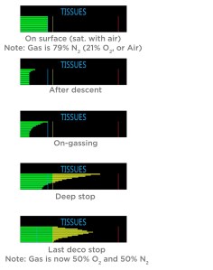
If you take a close look at the bottom two graphs (roughly corresponding to numbers (4) and (5)/(6) in fig. 5, you can see that the cyan line (representing P(ig)) has jumped a bit to the left. This change represents the drop in inspired inert gas pressure at the switch from bottom gas to deco gas. Fig. 5 shows the P(ig)s for both gases in a similar color.

All clear? For questions or comments, please feel free to drop me an email via my Contact page.

Stay safe and happy diving!